Abstract
Spatial transcriptomics technology captures gene expression profiles while preserving the spatial context of cells within tissues. Effectively integrating both gene expression and spatial information to identify distinct spatial regions and cluster cell subpopulations remains a fundamental challenge in data analysis. This paper introduces a novel cell clustering method for spatial transcriptomics that combines a variational autoencoder (VAE) with a graph neural network (GNN). The model employs a two-layer encoder with Simple Graph Convolution (SGC) at each level to produce low-dimensional embeddings. A decoder reconstructs the feature matrix, and the embeddings are refined by minimizing a reconstruction loss. These embeddings are then used for downstream clustering into cell subpopulations. Evaluated on multiple datasets, the proposed method outperforms several benchmark approaches in clustering accuracy and adaptability, demonstrating its effectiveness.
Introduction
Single-cell sequencing technology enables the measurement of genomes, transcriptomes, proteomes, and metabolomes at the individual cell level [1], thereby revealing information such as cell types, rare subtypes, functional states, and developmental trajectories. This provides more effective methods and approaches for disease diagnosis, treatment, and prevention. Furthermore, single-cell sequencing can explore intratumoral heterogeneity and the cellular microenvironment, uncover molecular mechanisms and subset characteristics of immune cells under various pathological conditions, and facilitate the development of more effective immunotherapeutic strategies [2].
Spatial transcriptomics technology enables the revelation of gene expression profiles in tissues or cells while preserving their spatial location information [3]. By performing high-resolution profiling of gene expression and retaining the spatial coordinates of sequenced cells, this approach facilitates the exploration of spatiotemporal dynamics in gene expression. Thereby, it enhances the understanding of cellular functions and tissue architecture, enables the study of cellular and tissue heterogeneity, and elucidates the mechanisms and progression of diseases [4]. Currently, multiple spatial transcriptomic technologies are available both domestically and internationally, such as Slide-seqV2 [5], LCM-seq [6], Stereo-seq [7], and 10x Visium [8].
Cell subpopulation clustering and spatial domain identification are crucial steps in spatial transcriptomics data analysis. Spatial domain identification and cell subpopulation clustering involve integrating spatial location information with gene expression profiles to identify cells with similar expression patterns under different physiological states, thereby inferring cell types and their interaction patterns [9]. Based on the identified spatial domains and cell subpopulations, it becomes possible to conduct studies such as characterizing gene expression patterns and gene enrichment, spatial spot deconvolution, reconstruction of cellular spatial locations, as well as investigating cell communication and gene interactions.
Currently, researchers worldwide have conducted a series of studies on spatial transcriptomic cell subpopulation clustering and spatial domain identification. For example, the Center for Genomics and Systems Biology at New York University released the Seurat toolbox [10] based on the R language, which streamlines the analysis pipeline for both single-cell sequencing and spatial transcriptomics data. It includes functions such as quality control, cell filtering, cell type identification, feature gene selection, differential expression analysis, and data visualization. The Institute of Computational Biology at the Helmholtz Center for Environmental Health in Germany introduced the Python-based Scanpy and Squidpy toolboxes [11-12], establishing an analytical ecosystem within Python for single-cell and spatial transcriptomics data. These tools support procedures such as data preprocessing, visualization, clustering, pseudotemporal analysis, trajectory inference, and differential expression analysis.
In both Seurat and Scanpy, the primary methods for cell subpopulation clustering and spatial domain identification are K-means [13] and Leiden [14], both of which are traditional clustering algorithms. mclust [15] is a Gaussian mixture model-based clustering method implemented in R; it performs effectively when processing data with diverse distributions. The Hidden Markov Random Field (HMRF) model [16] can effectively capture contextual spatial information of cells and achieve cell type identification through the construction of an energy function. The Fully Bayesian Statistical Model [17] defines a clustering objective function based on maximum likelihood estimation and performs clustering using weighted likelihoods across candidate cell subpopulation partitions. However, the aforementioned clustering methods consider only gene expression profiles and fail to incorporate spatial location information, resulting in limited accuracy in spatial domain identification and cell subpopulation clustering.
In recent years, graph deep learning has been recognized as an effective approach for analyzing spatial transcriptomics data [18]. Graph neural networks (GNNs) can fully leverage both gene expression profiles and spatial location information in spatial transcriptomic data, making them a powerful tool for improving the accuracy of cell subpopulation clustering. This paper proposes a cell subpopulation clustering method based on a variational autoencoder (VAE) and a graph neural network. Highly variable genes are selected from gene expression profiles to form a feature matrix, while spatial location information is used to compute Euclidean distances and construct an adjacency matrix. The feature matrix and adjacency matrix are processed by the variational autoencoder to generate low-dimensional embeddings. Downstream clustering methods are then applied to classify these embeddings into distinct cell subpopulations.
The variational autoencoder consists of an encoder and a decoder, both designed with a two-layer structure, each containing Simplified Graph Convolution (SGC) to produce low-dimensional representations. The proposed method was compared with several baseline approaches on commonly used spatial transcriptomic datasets, demonstrating superior clustering accuracy.
Methodology
Variational Graph Autoencoder (VGAE) in Cell Subpopulation Clustering
In the task of cell subpopulation clustering, the inputs to the Variational Graph Autoencoder (VGAE) are the feature matrix X, derived from gene expression profiles, and the adjacency matrix A, computed from spatial location information. A key aspect of the VGAE is its use of a two-layer graph neural network architecture to generate low-dimensional representations. The first graph neural network layer is used to compute a low-dimensional feature matrix X [19]:
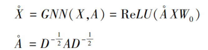
where  is the symmetrically normalized adjacency matrix, ReLU(·) = max(0, ·) denotes the rectified linear activation function, and W₀ represents the weight parameters of this graph neural network layer.
In the second graph neural network layer, the weight parameters W₁ are used to compute the mean and variance vectors of the feature matrix:
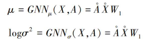
Here, the mean and variance vectors share the same set of weight coefficients. Based on this, the reparameterization trick [19] is applied to compute the low-dimensional representation:
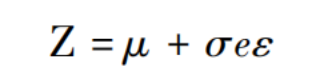
Finally, the loss function comprises two types of errors. The first is the reconstruction error, which measures the similarity between the input and output adjacency matrices. The second type of error aims to minimize the discrepancy between the initial label distribution q and the predicted label distribution p. The mathematical expression of the loss function is as follows:

where KL(·) denotes the Kullback-Leibler divergence between two probability distributions. Finally, downstream clustering is performed on the generated low-dimensional representations to obtain cell subpopulation clustering labels. The clustering labels are compared against the gold standard to validate the accuracy of the clustering method.
Graph Neural Network
This paper incorporates Simplified Graph Convolution (SGC) into the variational autoencoder to compute low-dimensional representations. SGC modifies the original Graph Convolutional Network (GCN) [20] to reduce model complexity and redundant computations. It simplifies the computational process and improves efficiency by collapsing weight matrices between successive layers and removing non-linearities. This simplified linear model has been theoretically and empirically demonstrated to achieve better performance, with its convolutional kernel modified into a linear pattern:
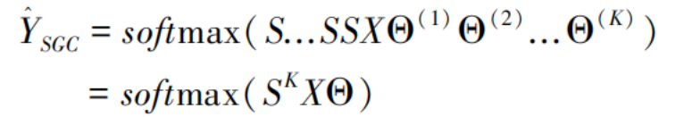
where S is the normalized adjacency matrix, X denotes the feature matrix, Θ represents the weight matrix, and softmax refers to the normalized exponential function.
Spatial Transcriptomics Validation Dataset
This study employs one of the most widely used spatial transcriptomics datasets to validate the accuracy of the cell subpopulation clustering algorithm. The dataset pertains to the human dorsolateral prefrontal cortex (DLPFC), with raw data available from the 10x Visium data repository. It includes gene expression profiles, spatial location information, and histological images. The corresponding gold standard annotations for cell subpopulations can be accessed via the SpatialLIBD project [21].
The dataset comprises 12 tissue sections, with the number of captured spots per section ranging from 3,460 to 4,789, and a total of 33,538 genes sequenced. The samples are labeled from 151507 to 151676. In manual annotations, each sample contains five or seven cell subpopulations, including two major cell types: DLPFC layers and white matter. Each cell subpopulation exhibits clear boundaries, making this dataset highly suitable for evaluating clustering accuracy. The proposed clustering method is compared with multiple baseline methods on this dataset to assess their clustering performance. Furthermore, since the cell subpopulations in each sample are arranged in chronological order, this dataset is also appropriate for spatial trajectory inference evaluation.
Evaluation Metrics
When manually annotated labels are available for spatial transcriptomics datasets, the Adjusted Rand Index (ARI) can be used to evaluate the accuracy of cell subpopulation clustering. Since the human dorsolateral prefrontal cortex (DLPFC) dataset used in this study comes with gold standard annotations, the ARI is computed by comparing the predicted labels against these gold standard labels. Let P = {P₁, P₂, …, Pₖ} and G = {G₁, G₂, …, Gₗ} represent the predicted labels and the manually annotated labels, respectively. The Adjusted Rand Index can be calculated using the following formula:
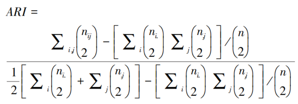
Here, c represents the number of cell subpopulations, nᵢ and nⱼ denote the number of cells belonging to the k-th predicted label category and the l-th manual annotation label category, respectively, while nᵢⱼ indicates the number of cells that belong to both the k-th predicted label category and the l-th manual annotation label category. The Adjusted Rand Index ranges from [0, 1]. In this study, it is computed using the adjusted_rand_score function from the scikit-learn toolkit. A higher ARI value indicates higher accuracy in cell subpopulation clustering.
Selection of Neural Network Hyperparameters
The clustering method based on the variational autoencoder was implemented in Python using PyTorch and the PyTorch Geometric (PyG) library [22]. Initially, gene expression profiles were normalized and log-transformed via the Scanpy toolbox [23], from which 3,000 highly variable genes were selected to construct the feature matrix. The adjacency matrix was then generated using the k-nearest neighbors algorithm (with k = 6) from the scikit-learn package [24], identifying spatial neighbors for each cell. Both the feature matrix and adjacency matrix were input into the variational autoencoder to produce low-dimensional embeddings. Key hyperparameters were configured as follows: the input dimension was set to 3,000 (number of highly variable genes), the hidden dimension to 128, and the output dimension to 30. The learning rate was set at 1×10⁻⁴, with 5,000 iterations for training. Weight decay was set to 1×10⁻⁴, gradient clipping was applied at a threshold of 5, and a random seed of 0 was used for reproducibility. The model architecture incorporated 4 hidden layers, each employing the Exponential Linear Unit (ELU) activation function. All experiments were performed on a hardware system running Ubuntu 20.04.5 LTS, equipped with an i9-12900F CPU, 64 GB of RAM, and an NVIDIA GeForce RTX™ 3090 Ti GPU.
After obtaining the low-dimensional embeddings, the traditional K-means clustering method was applied to cluster cell subpopulations, implemented via the scikit-learn package. In the K-means method, the number of cell subpopulations was set to match the number of categories in the gold standard, yielding predicted cell subtype labels. Finally, the Adjusted Rand Index (ARI) was calculated based on the predicted labels and the manual annotations, and the ARI values were compared to evaluate the accuracy of each method. The benchmark methods used in this study include Scanpy [23], SpaGCN [25], SEDR [26], STAGATE [27], DeepST [28], and BayesSpace [29], all of which represent state-of-the-art graph neural network-based algorithms for spatial transcriptomics cell subpopulation clustering and spatial domain identification.
Results
Clustering Accuracy Comparison
The proposed cell subpopulation clustering and spatial domain identification method is named VGAE_SGC. To demonstrate its accuracy and effectiveness, VGAE_SGC was compared against six spatial clustering benchmark methods: Scanpy, SpaGCN, SEDR, STAGATE, DeepST, and BayesSpace. All seven methods were evaluated on the human dorsolateral prefrontal cortex (DLPFC) spatial transcriptomics dataset. The Adjusted Rand Index (ARI) was computed for each method across all 12 tissue sections, and the average ARI value was derived.
As shown in Fig. 1, which presents the average ARI values of each method on the Human DLPFC data, the proposed VGAE_SGC method achieved the highest ARI value of 0.539. Among the seven methods, three exceeded an ARI of 0.5: VGAE_SGC, DeepST, and STAGATE. In contrast, Scanpy, which uses the traditional Leiden algorithm for cell subpopulation clustering and does not incorporate spatial location information, yielded the lowest average ARI value of 0.311. The accuracies of SpaGCN, SEDR, and BayesSpace fell within an intermediate range, with ARI values around 0.45. These results indicate that the proposed method outperforms existing cell subpopulation clustering approaches in terms of clustering accuracy.
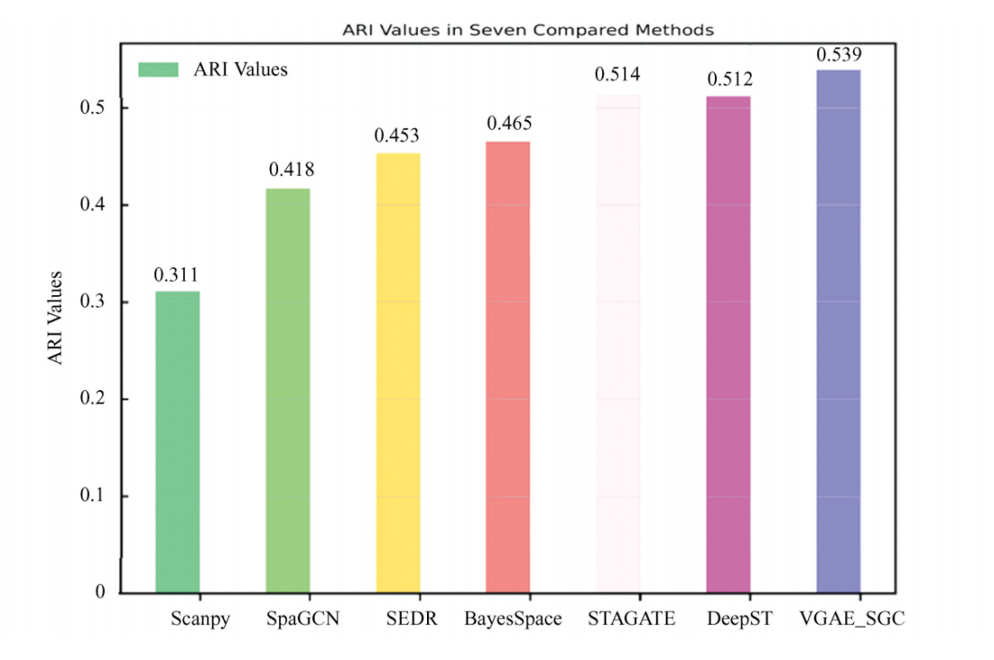
Fig.1 Average ARI values for cell clustering of spatial transcriptomics
Spatial Domain Identification Results Comparison
To further demonstrate the superiority of VGAE_SGC in spatial domain identification, a single sample from the Human DLPFC dataset was selected to illustrate the spatial domain recognition results of all seven methods. Sample 151675 was chosen for detailed visualization, and Fig. 2 shows the cell subpopulation clustering results for each method on this sample. The gold standard for this sample comprises seven spatial domains with clearly defined boundaries, arranged in a specific temporal sequence.
On this sample, the proposed VGAE_SGC method again achieved the highest ARI value of 0.550. None of the other six benchmark methods exceeded an ARI of 0.50, underscoring the clustering advantage of VGAE_SGC in this case. In terms of spatial domain recognition, the results of VGAE_SGC and DeepST most closely resembled the gold standard, with clearly demarcated boundaries between all spatial domains. In contrast, SpaGCN and Scanpy—which yielded lower ARI values—exhibited poorly defined spatial domains with disorganized cell distributions. Fig. 2 illustrates that the proposed VGAE_SGC method more effectively leverages spatial location information to accurately localize cells and identify spatial domains.
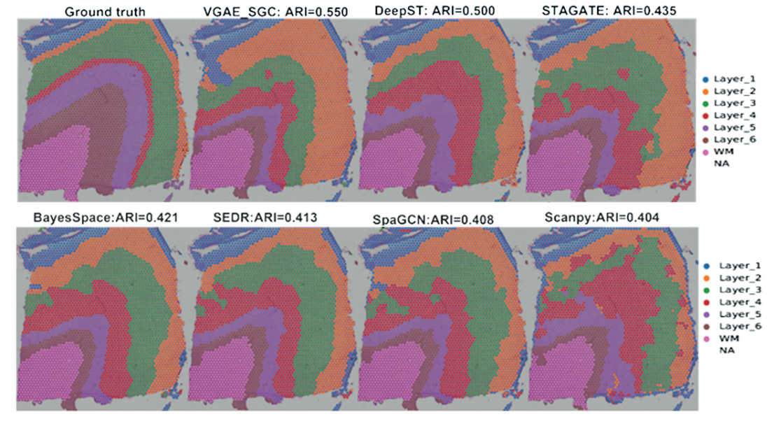
Fig.2 Spatial domain identification results of seven compared methods for spatial transcriptomics
Low-Dimensional Representation Quality Comparison
Among the seven methods compared in this study, low-dimensional representations could be obtained from four of them, enabling the visualization of reduced-dimensional clustering patterns. This section compares the quality of the low-dimensional embeddings generated by four methods: VGAE_SGC, DeepST, STAGATE, and SEDR. The corresponding dimensionality reduction plots are shown in Fig. 3. First, VGAE_SGC achieved the highest Adjusted Rand Index (ARI) of 0.550. DeepST performed closely to VGAE_SGC with an ARI of 0.50. Their UMAP visualizations also appeared similar: each cell subpopulation was distinctly separated and spatially arranged in a meaningful sequence. In contrast, the dimensionality reduction results of STAGATE and SEDR were less satisfactory. For instance, in STAGATE, Layer_1 and Layer_2 overlapped considerably, while SEDR showed disorganized and poorly separated cell subpopulations without clear spatial or structural ordering. These results suggest that STAGATE and SEDR did not adequately integrate gene expression profiles with spatial location information during clustering. In summary, compared to existing benchmark methods for spatial transcriptomic cell subpopulation clustering, the results from these three aspects demonstrate the accuracy and effectiveness of the proposed VGAE_SGC method.
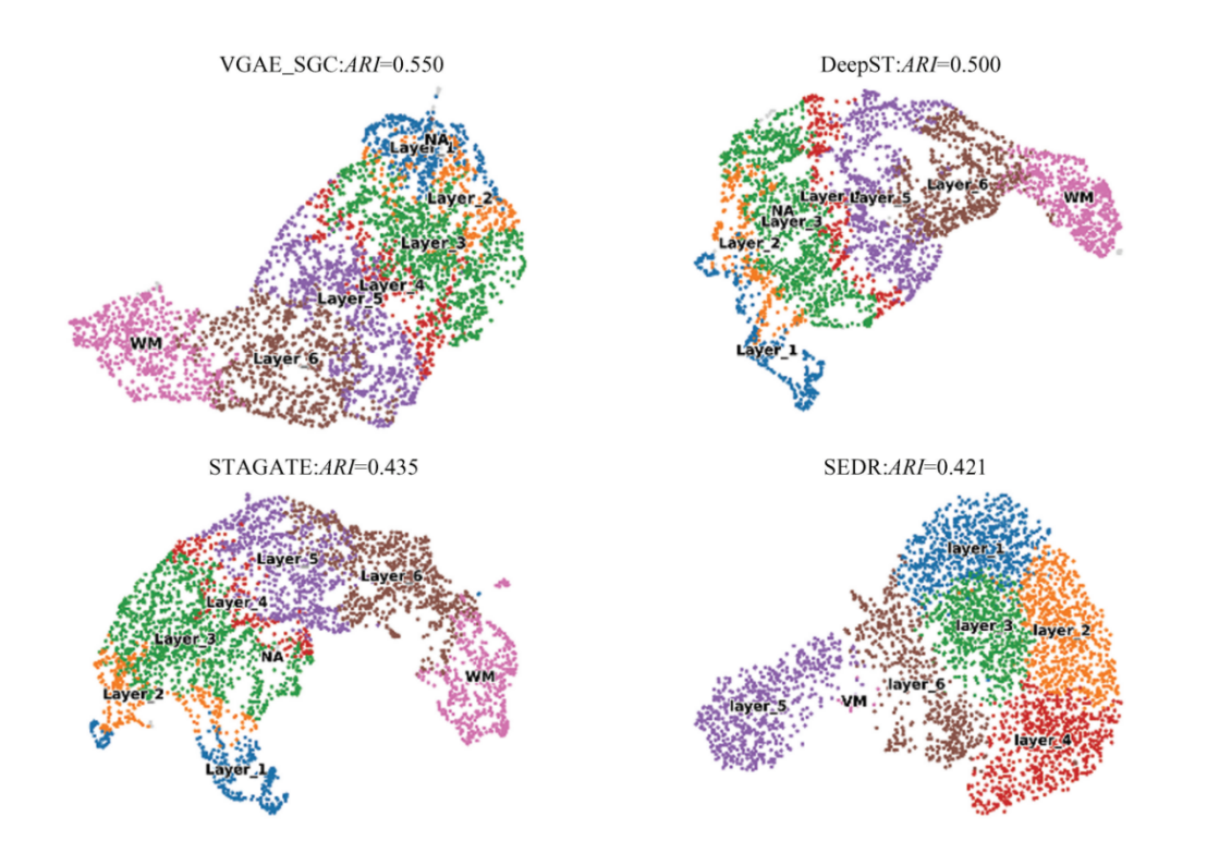
Fig.3 The Umap diagram of latent embedding in four methods
Discussion
Utilizing graph deep learning to integrate gene expression profiles and spatial location information in spatial transcriptomics can effectively improve the accuracy of cell subpopulation clustering. In this study, we propose a spatial transcriptomics clustering framework named VGAE_SGC, which embeds a simplified graph convolution within a variational autoencoder to process both gene expression profiles and spatial location information. Compared with multiple benchmark methods on the human dorsolateral prefrontal cortex (Human DLPFC) spatial transcriptomics dataset, VGAE_SGC demonstrates advantages in three aspects: the accuracy of cell subpopulation clustering, the identification of spatial domains, and the quality of low-dimensional representations. These results validate the effectiveness of the proposed variational autoencoder-based spatial transcriptomics cell subpopulation clustering method.
References
[1] NAWY T. Single-cell sequencing [J]. Nature Methods, 2014, 11(1): 18–18. DOI:10.1038/nmeth.2771.
[2] LU Ting. Bioinformatics analysis for gene differential expression [J]. Chinese Journal of Bioinformatics, 2014, 12(2): 140–144. DOI:10.3969/j.issn.1672-5565.2014.02.20140210.
[3] XU Xing, CAI Linfeng, ZHANG Qiannan, et al. Advances in single-cell and spatial transcriptome analysis [J]. Journal of Analytical Testing, 2022, 41(9): 1322–1334. DOI:10.19969/j.fxcsxb.22052401.
[4] WILLIAMS C G, LEE H J, ASATSUMA T, et al. An introduction to spatial transcriptomics for biomedical research [J]. Genome Medicine, 2022, 14(1): 1–18. DOI:10.1186/s13073-022-01075-1.
[5] RODRIQUES S G, STICKELS R R, GOEVA A, et al. Slide-seq: A scalable technology for measuring genome-wide expression at high spatial resolution [J]. Science, 2019, 363(6434): 1463–1467. DOI:10.1126/science.aaw1219.
[6] NICHTERWITZ S, CHEN G, AGUILA BENITEZ J, et al. Laser capture microscopy coupled with Smart-seq2 for precise spatial transcriptomic profiling [J]. Nature Communications, 2016, 7(1): 12139. DOI:10.1038/ncomms12139.
[7] XIA Keke, SUN Haixi, LI Jie, et al. Single-cell Stereo-seq enables cell type-specific spatial transcriptome characterization in Arabidopsis leaves [J]. bioRxiv, 2021: 2021.10.20.465066. DOI:10.1101/2021.10.20.465066.
[8] RAO N, CLARK S, HABERN O. Bridging genomics and tissue pathology: 10x Genomics explores new frontiers with the Visium spatial gene expression solution [J]. Genetic Engineering & Biotechnology News, 2020, 40(2): 50–51. DOI:10.1089/gen.40.02.16.
[9] WANG Lin, ZHAO Guihua. Statistical methods for spatially resolved transcriptomic data analysis [J]. Bioprocess, 2023, 13: 57. DOI:10.12677/BP.2023.131008.
[10] SATIJA R, FARRELL J A, GENNERT D, et al. Spatial reconstruction of single-cell gene expression data [J]. Nature Biotechnology, 2015, 33(5): 495–502. DOI:10.1038/nbt.3192.
[11] WOLF F A, ANGERER P, THEIS F J. SCANPY: Large-scale single-cell gene expression data analysis [J]. Genome Biology, 2018, 19: 1–5. DOI:10.1186/s13059-017-1382-0.
[12] PALLA G, SPITZER H, KLEIN M, et al. Squidpy: A scalable framework for spatial omics analysis [J]. Nature Methods, 2022, 19(2): 171–178. DOI:10.1038/s41592-021-01358-2.
[13] SONG Dongqi, SONG Yuqing, LIU Zhe, et al. Novel model clustering approach for gene expression data [J]. Computer and Applied Chemistry, 2015, 32(1): 71–74. DOI:10.3390/diagnostics10080584.
[14] TRAAG V A, WALTMAN L, VAN ECK N J. From Louvain to Leiden: Guaranteeing well-connected communities [J]. Scientific Reports, 2019, 9(1): 5233. DOI:10.1038/s41598-019-41695-z.
[15] HAUGHTON D, LEGRAND P, WOOLFORD S. Review of three latent class cluster analysis packages: Latent GOLD, poLCA, and MCLUST [J]. The American Statistician, 2009, 63(1): 81–91. DOI:10.1198/tast.2009.0016.
[16] CHATZIS S P, TSECHPENAKIS G. The infinite hidden Markov random field model [J]. IEEE Transactions on Neural Networks, 2010, 21(6): 1004–1014. DOI:10.1109/TNN.2010.2046910.
[17] MO Qianxing, SHEN Ronglai, GUO Cui, et al. A fully Bayesian latent variable model for integrative clustering analysis of multi-type omics data [J]. Biostatistics, 2018, 19(1): 71–86. DOI:10.1093/biostatistics/kxx017.
[18] WANG Guoli, SUN Yu, WEI Benzheng. Systematic review on graph deep learning in medical image segmentation [J]. Computer Engineering and Applications, 2022, 58(12): 37–50. DOI:10.3778/j.issn.1002-8331.2112-0225.
[19] KIPF T N, WELLING M. Variational graph auto-encoders [J]. arXiv preprint arXiv:1611.07308, 2016. DOI:10.48550/arXiv.1611.07308.
[20] ZHANG Si, TONG Hanghang, XU Jiejun, et al. Graph convolutional networks: A comprehensive review [J]. Computational Social Networks, 2019, 6(1): 1–23. DOI:10.1186/s40649-019-0069-y.
[21] PARDO B, SPANGLER A, WEBER L M, et al. SpatialLIBD: An R/Bioconductor package to visualize spatially resolved transcriptomics data [J]. BMC Genomics, 2022, 23(1): 1–5. DOI:10.1186/s12864-022-08601-w.
[22] FEY M, LENSSEN J E. Fast graph representation learning with PyTorch Geometric [J]. arXiv preprint: 1903.02428, 2019. DOI:10.48550/arXiv.1903.02428.
[23] WOLF F A, ANGERER P, THEIS F J. SCANPY: Large-scale single-cell gene expression data analysis [J]. Genome Biology, 2018, 19(1): 1–5. DOI:https://doi.org/10.1186/s13059-017-1382-0.
[24] PEDREGOSA F, VAROQUAUX G, GRAMFORT A, et al. Scikit-learn: Machine learning in Python [J]. The Journal of Machine Learning Research, 2011, 12: 2825–2830. DOI:10.48550/arXiv.1201.0490.
[25] HU Jian, LI Xiangjie, COLEMAN K, et al. SpaGCN: Integrating gene expression, spatial location and histology to identify spatial domains and spatially variable genes by graph convolutional network [J]. Nature Methods, 2021, 18(11): 1342–1351. DOI:10.1038/s41592-021-01255-8.
[26] FU Huazhu, XU Hang, CHONG K, et al. Unsupervised spatially embedded deep representation of spatial transcriptomics [J]. bioRxiv, 2021: 2021.06.15.448542. DOI:10.1101/2021.06.15.448542.
[27] DONG Kangning, ZHANG Shihua. Deciphering spatial domains from spatially resolved transcriptomics with an adaptive graph attention auto-encoder [J]. Nature Communications, 2022, 13(1): 1739. DOI:10.1038/s41467-022-29439-6.
[28] XU Chang, JIN Xiyun, WEI Songren, et al. DeepST: Identifying spatial domains in spatial transcriptomics by deep learning [J]. Nucleic Acids Research, 2022, 50(22): e131–e131. DOI:10.1093/nar/gkac901.
[29] ZHAO E, STONE M R, REN Xing, et al. Spatial transcriptomics at subspot resolution with BayesSpace [J]. Nature Biotechnology, 2021, 39(11): 1375–1384. DOI:10.1038/s41587-021-00935-2.